
Solving the Heat Equation in a Microprocessor
During 2020-2021, I decided to take the Computational Physics module in which I learned more aboout numerical algorithms and efficiency. As part of the final coursework, I had to simulate the temperature distribution that developed inside a microprocessor running at full speed. I then had to investigate how to get the temperature below the operating value of $80C^o$ by mean of a heat sink and forced convection (i.e. a fan). .
A look at the system
The system I simulated looked like that:
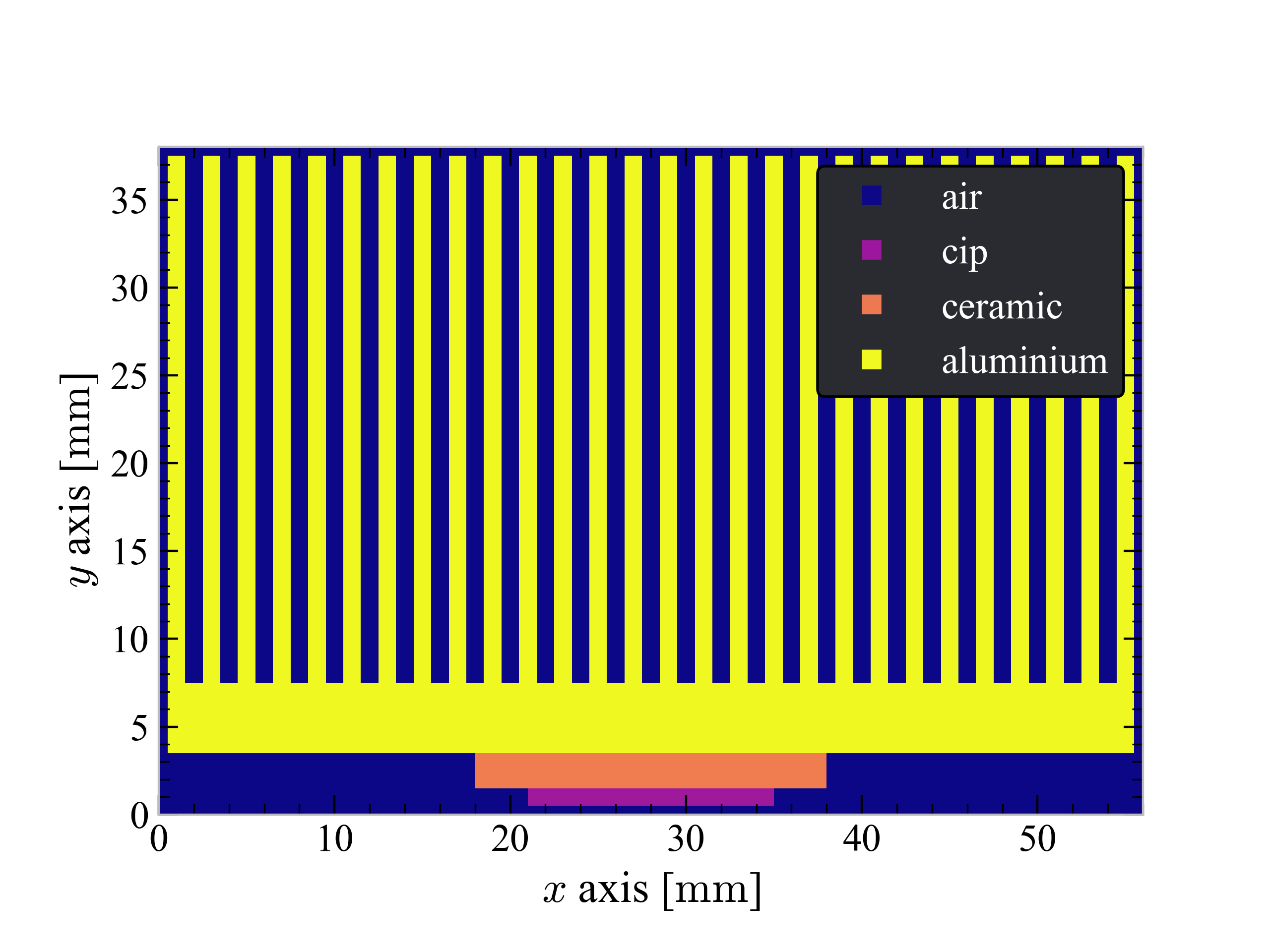
The microprocessor is positioned on the bottom (purple) and it is substained by a ceramic casing (orange). An alluminium heat sink could be optionally added to improve the dispersive capability of the system. As you can probably tell, I modelled the system dividing it into pixels, each one with its own temperature and capable of exchanging heat with the 4 nearest neighbours.
The Maths
The core of the project reduced to solve numerically the steady state sourced heat equation, which by taking ($\partial T / \partial t = 0$) turns into:
\[k\nabla^2 T(x,y) = -q(x,y)\]where,
- $T$ is the temperature as a function of position x,y;
- $k$$ is the thermal conductivity
- $q$ is the power density
Which is a partial differential equation (PDE). In the system, energy was produced inside the microchip (power density $q$), and it was dissipated at the system-air interface thus defining the boundary conditions of the problem. In particular, we considered two cases: natural convection, where air circulates due to spontaneous convection cycles and forced convection, where air was forced through the system via a fan. Empirical expressions for the heat flux at the interface with air was given to us to use in both scenarios.
By labelling each pixel in the system $i,j$ and by denoting their (square) size with the letter $h$, we can take a finite difference approach and rewrite the differential equation for a pixel in the bulk material as:
\[\kappa_{i,j} \frac{-4T_{i,j}+T_{i+1,j}+T_{i-1,j}+T_{i,j+1}+T_{i,j-1}}{h^2}=-q_{i,j}\]Of course, this assumes that all the surrounding pixels have the same thermal conductivity $\kappa$ and this is obviously not the case since the system is etherogeneous and made by different materials. Hence, the above differential equation changes slightly depending on whether the nearest neighbours are ‘air’ or if they have a different thermal conductivity. If you are interested, more details of this, including a worked example, can be found in the lab report (button above).
The punch line is that there is one such discrete equation for every pixel in the microprocessor and hence there are $N$ unknown temperatures and $N$ equations: this system can be solved! The system of equations above can be written more compactly in matrix form:
\[\underline{\underline{M}} T = b_{(T)}\]where $\underline{\underline{M}}$ is a matrix which depends not on $T$ and $b_{(T)}$ is a vector that depends on temperature and that encapsulates all the non-linearity arising in the pixels at the matter-air interface. Indeed, the heat flux exiting the system is modelled as not being linear with temperature.
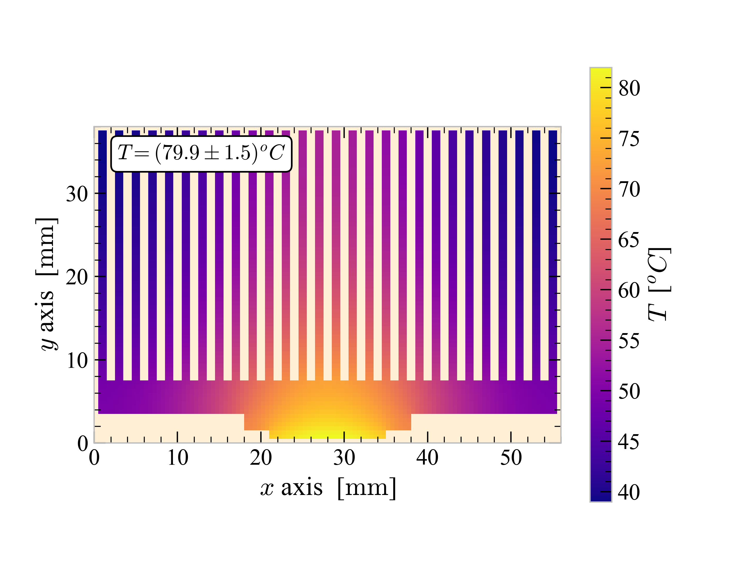
This image shows the solution of the temperature map under forced convection boundary conditions. The temperature rated on the top left corner refers to the average temperature across the microprocessor.
How to solve this
The last equation I wrote needs to be solved for temperature. If the vector $b_{(T)}$ did not depend on temperature, the game would be easy. By inverting the matrix $M$ (by one of the several developed algorithms), the solution is found to be
\[T = M^{-1} b\]As shown in the report (button top of the page), this happens to be the case for forced convection boundary conditions. We call this method ‘Direct method’ for future reference. However, in the natural convection BC case, $b$ depends on time and this complicates things.
A “quick and dirty” approach: Relaxation method
One to solve the above is taking an arbitrary initial guess $T^{(0)}$ and calculate $b(T^{(0)})$ using that. Then we try to update the temperature in the following way
\(T^{(n+1)}=M^{-1} T^{(n)}\),
hoping for the temperature to converge. This method can be very slow, depending on the problem, however the good news is that the most computationally expxensive operation, which is inverting the matrix $M$, needs to be performed only once.
Newton’s method
Netwon’s method is an algorithm to solve systems of simultaneous non-linear equations. What makes it potentially more powerful than the relaxation method above is that netwon’s algorithm uses an extra piece of information: the gradient.
In order to make this concept clearer, let’s get an actual example: Consider a system made by 3 pixels labelled by $i=0,1,2$, then there will be three equations to simultaneously solve. By bringing all the terms on the left hand side, we can write:
\[f_1(T_1, T_2, T_3) = 0\] \[f_2(T_1, T_2, T_3) = 0\] \[f_3(T_1, T_2, T_3) = 0\]Netwon’s method is a root finder methods: it finds the values of $T_i$ for which all the above are $0$. It assumes that the jacobian
\(J_{ij} = \frac{\partial f_i}{\partial T_j}\),
is known. It turns out that in our particular problem, expressions for the derivatives of $f_i$ could be found analytically. See the appendix at the end of this page for an outline of the Netwon’s root-finding method.
The substantial difference with Relaxatoin is that the last one only uses the values of the function $f_i$ evaluated for a given vector of $T$ values. Newton’s method uses more information, including derivatives of $f_i$.
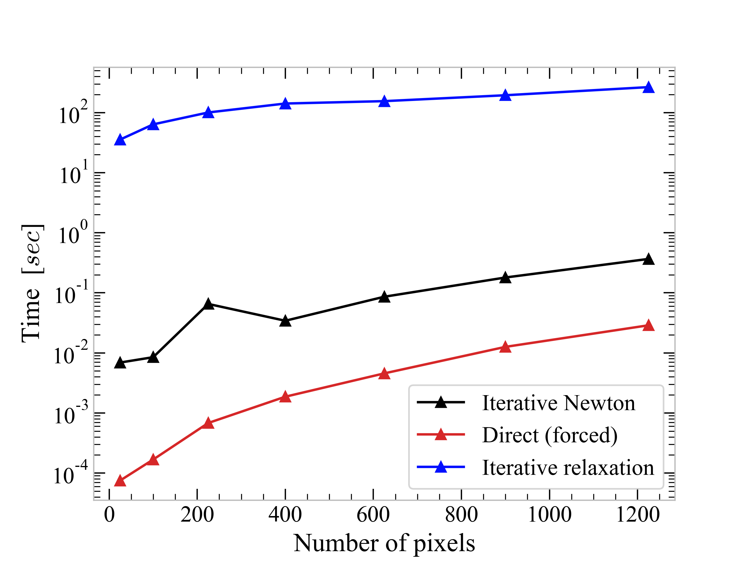
The consequences on the number of required iterations to reach convergence in this case is dramatic. Studying the maximum temperature in the microprocessor (violet in Fig. 1), we see that in order to achieve a fractional change of $10^{-8}$ with the relaxation method, we need to perform $O(1000)$ iterations. Newton’s method only takes $O(10)$. A comparison of relaxation method (iterative), netwon’s method (itearative) an direct method (non-iterative) is shown in the image below. It is clear that Newton’s method outperforms the relaxation one over a wide range of pixel numbers. However for linear systems, we found that the direct method still remains the fastest one within the tested range.
Conclusion
The take away is that sometimes it is worth to look for something one step more complicated than the easiest solutoin. If I had been working with the relaxation method only, I would have never managed to get all the results: the algorithm took minutes to run, making the debugging slow to progress. Spending some to develop an alternative route than the one suggested by the lab script and developing the netwon’s root finding approach turned out to be an investment, cutting the running time to orders of magnitude.
Appendix: Newtons’s Method
So, how does this method work? Let’s start with an easy example: say that we have a system of two equations and two unknowns $(x,y)$. This system can be always rewritten as:
\[f(x,y)=0\] \[g(x,y)=0\]Hence, the problem of solving it turns into a root finding problem. Additionally, say that we know the values of the two functions at a point of coordinate $\mathbf{q_0} = (x_0,y_0)$. Then we can use a linear taylor expansion to find the value of the function at $(x_0+\delta_{x0}, y_0+\delta_{y0})$:
\[f(y_0+\delta_{y0}, y_0+\delta_{y0}) \approx f(x_0,y_0)+\left.\frac{\partial f}{\partial x}\right|_{x_0,y_0} \delta_{x0} + \left.\frac{\partial f}{\partial y}\right|_{x_0,y_0} \delta_{y0} + O(\delta^2)\] \[g(y_0+\delta_{y0}, y_0+\delta_{y0}) \approx g(x_0,y_0)+\left.\frac{\partial g}{\partial x}\right|_{x_0,y_0} \delta_{x0} + \left.\frac{\partial g}{\partial y}\right|_{x_0,y_0} \delta_{y0} + O(\delta^2)\]The whole point is that we want to do a step $(\delta_x,\delta_y)$ such that the left hand side vanishes. Hence, we set it to $0$ in the above and we solve for the step size. Rewritten in matrix notation, this corresponds to:
\[\begin{bmatrix} \left.\frac{\partial f}{\partial x}\right|_{x_0,y_0} & \left.\frac{\partial f}{\partial y}\right|_{x_0,y_0} \\ \left.\frac{\partial g}{\partial x}\right|_{x_0,y_0} & \left.\frac{\partial g}{\partial y}\right|_{x_0,y_0} \\ \end{bmatrix} \begin{bmatrix} \delta_{x0} \\ \delta_{y0} \end{bmatrix} = - \begin{bmatrix} f(x_0,y_0) \\ g(x_0,y_0) \end{bmatrix}\]By inverting the (Jacobian) matrix that we label with letter $\mathbf{J_0}$, the vector $\mathbf{\sigma_0}$ can be found. Then, the new values of $\mathbf{x}=(x,y)$ are found by doing:
\(\mathbf{x_1} = \mathbf{x_0} + \mathbf{\sigma_0} = \mathbf{x_0} - \mathbf{J_{0}^{-1}} \mathbf{f_{(x_0,y_0)}}\) .
More generally, the update rule is:
\(\mathbf{x_{n+1}} = \mathbf{x_n} - \mathbf{J_{n}^{-1}} \mathbf{f_{(x_n,y_n})}\) .
References
[1] Mark Newmann, Computational Physics