
What connects a Rolls Royce engine, a neural network and a quantum computer? keep reading and you are going to find out!
Between the 28th-29th July 2022 I took part in the Quantum Computing Hackathon organised by the National Quantum Computing Center (NQCC) in the UK. The experience was a blast, with people from many countries coming together in teams to solve real world problems using quantum computing. Each of the 9 teams had to tackle a different problems, and our was provided by Rolls Royce. After developing our algorithm, we present it to a jury of experienced researchers, and we managed to win the second prize at the hackathon.
The whole experience was an amazing opportunity to meet many passionate students in the field of Quantum Computing across Europe, as well as QC professionals working in different fields. In the next sections you can learn more about what we have done and our results.
The Problem
Our “end-user” (aka Rolls Royce) gave us an engine dataset with the purpose of learning Remaining Useful Life (RUL). The dataset is the NASA Turbofan Jet Engine dataset (kaggle), which contains several sensor measurements collected on engines which are let run until they break down.
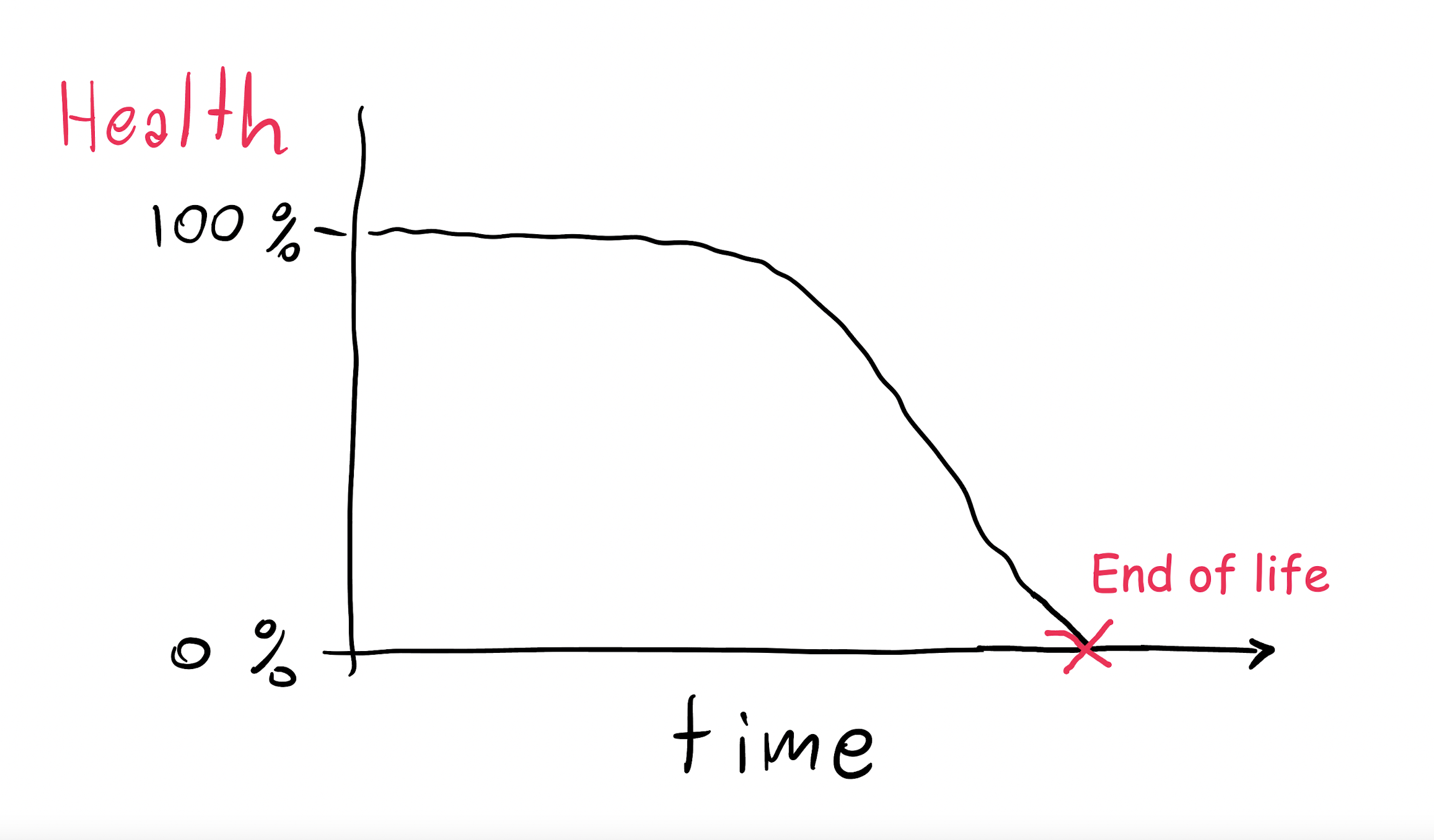
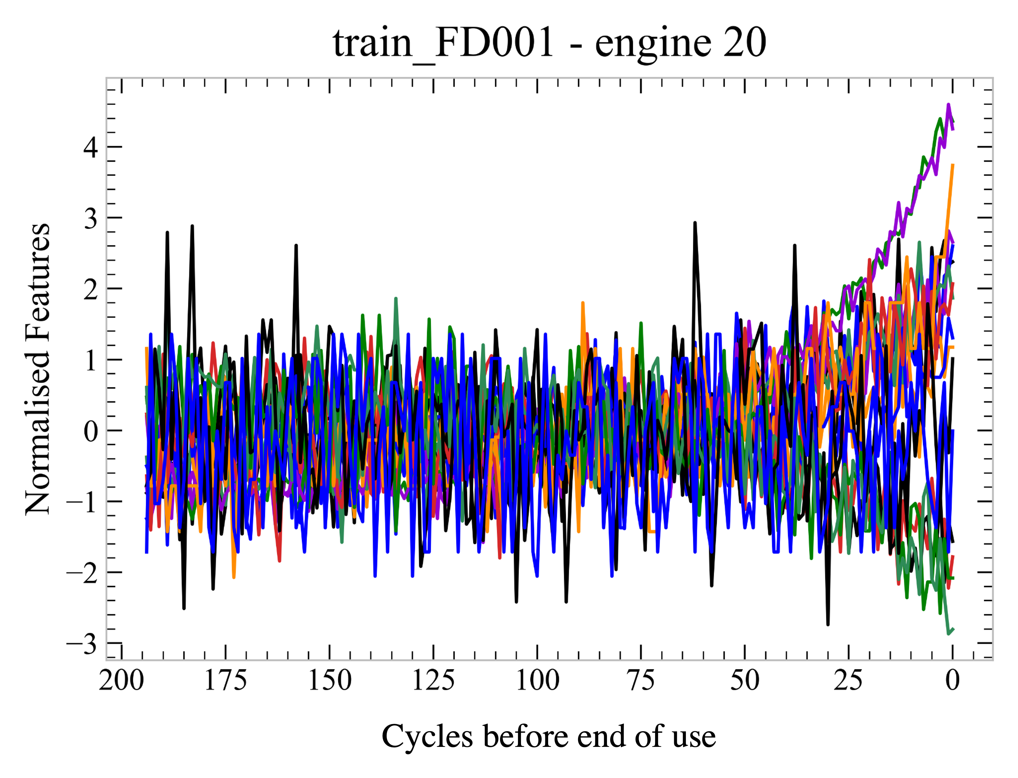
Our task was to use these data to predict how long before an engine breaks down. This is not a trivial task, as the data are quite noisy and it is not obvious which information is relevant. Moreover, a single sensor’s readings showed great variability across several engine datasets. Because of these issues, we though that a machine learning approach would be a good fit for the problem.
A Classical Approach: RNN
This type of time-aligned data is known as a time series. When choosing a classical machine learning approach, we wanted to pick an algorithm that exploited the fact that data have an order. Therefore, we came to the decision of using a Recurrent Neural Network (RNN) to do so.
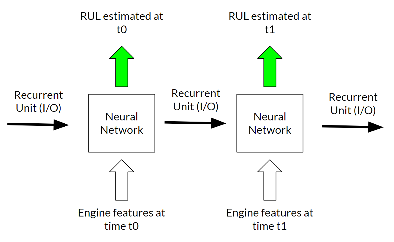
In a standard Neural Network, the input features (sensor measurements) are passed to the model, that performs some calculation to produce an output (in this case the RUL prediction). In a recurrent neural network, an extra output is produced via some neurons that we call recurrent neurons. This output is then passed together with the features from the following time step into the same RNN model. The recurrent neurons have the duty of conveying information about the previous time steps in order to improve the predictions at later times.
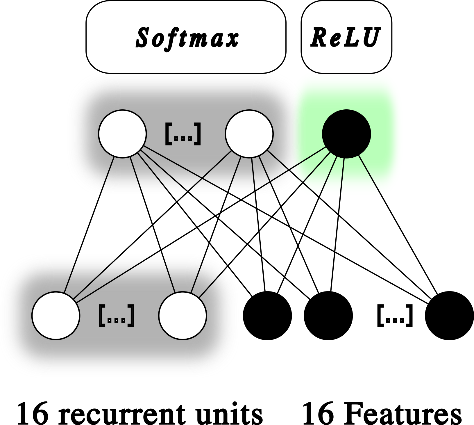
The image below shows our implementation of the RNN. The model is quite simple, it does not have any hidden layer, but it offers a baseline benchmark for the quantum approach that we investigate later. Note the choice of the activation functions. The RUL is an integer positive number: it tells how many cycles the engine can run before breaking down. Therefore, we chose ReLU as activation function, that only produces positive numbers from zero to infinity. The recurrent neurons are kept between 0 and 1 by the application of the softmax function.
Going Quantum: QB-RNN
After all, we were at a Quantum Hackathon, not a classical machine-learning Hackathon. The task of predicting RUL with a RNN is well established; how could we use a Quantum Computer to do the same? From the start, we thought about implementing a Quantum Machine Learning algorithm, however finding the right one was far from obvious. Initially we though about some very fancy ones, such as the Recurrent Quantum Neural Network developed by Bausch (Recurrennt Quantum Neural Networks, 2020).
Eventually, we had to readjust our expectations according to the possibilities of the early quantum computers that are currently available. We were given access to the Lucy quantum computer, developed by Oxford Quantum Circuits (OQC) and made available through Amazon Web Service (AWS). Lucy has 8 qubits, and its levels of noise does not allow for high number of gates to be operated one after the other.
Therefore we designed an algorithm that played around these limitations. We created a classic-quantum hybrid recurrent neural network that we named Quantum Boosted Recurrent Neural Network (QB-RNN).
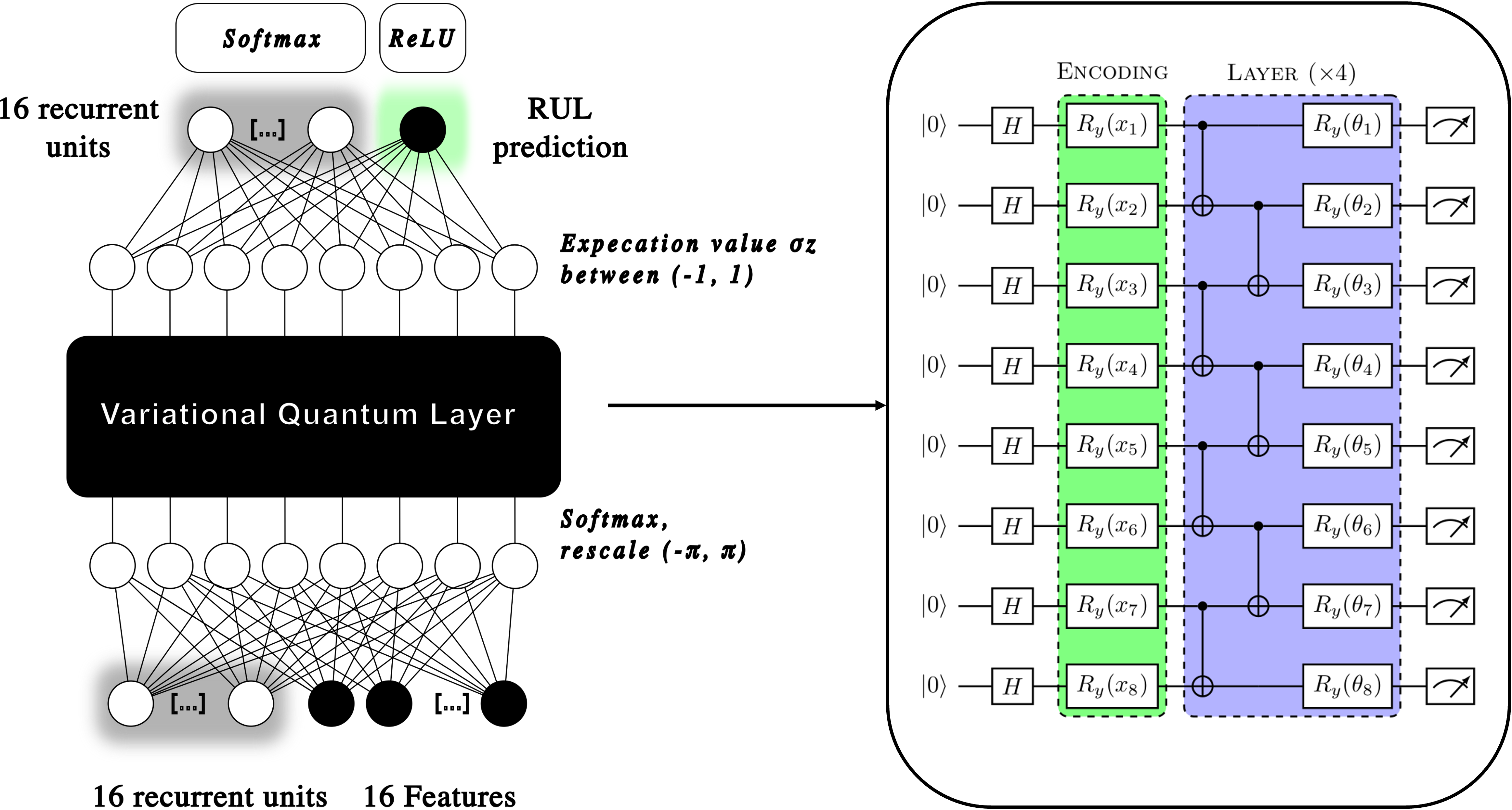
As the picture shows, we used an encoding layer to map the 32 input features into 8 features, as the number of qubits that were available to us. These were then rescaled between $(-\pi, \pi)$ to encode a single-qubit rotation on the bloch sphere, which is the way that the input is encoded into the quantum circuit. The circuit is then run multiple times (1000) in order to estimate the expectation value of the $\sigma_z$ operator at the output of the circuit on each individual qubit. These 8 expectation values are then moved back to the classical neural network and propagated to compute the next recurrent units and the RUL prediction.
Results
We now give a look at the results for the two networks and we compare them. Both the RNN and QB-RNN were trained on 1000 engine data, sampled randomly from a pool of 100 engines in the training set. The QB-RNN was trained using a simulator that emulates the behaviour of the quantum circuit, however we decided also to try and use the trained model on Lucy (the quantum computer) to try and make predictions.
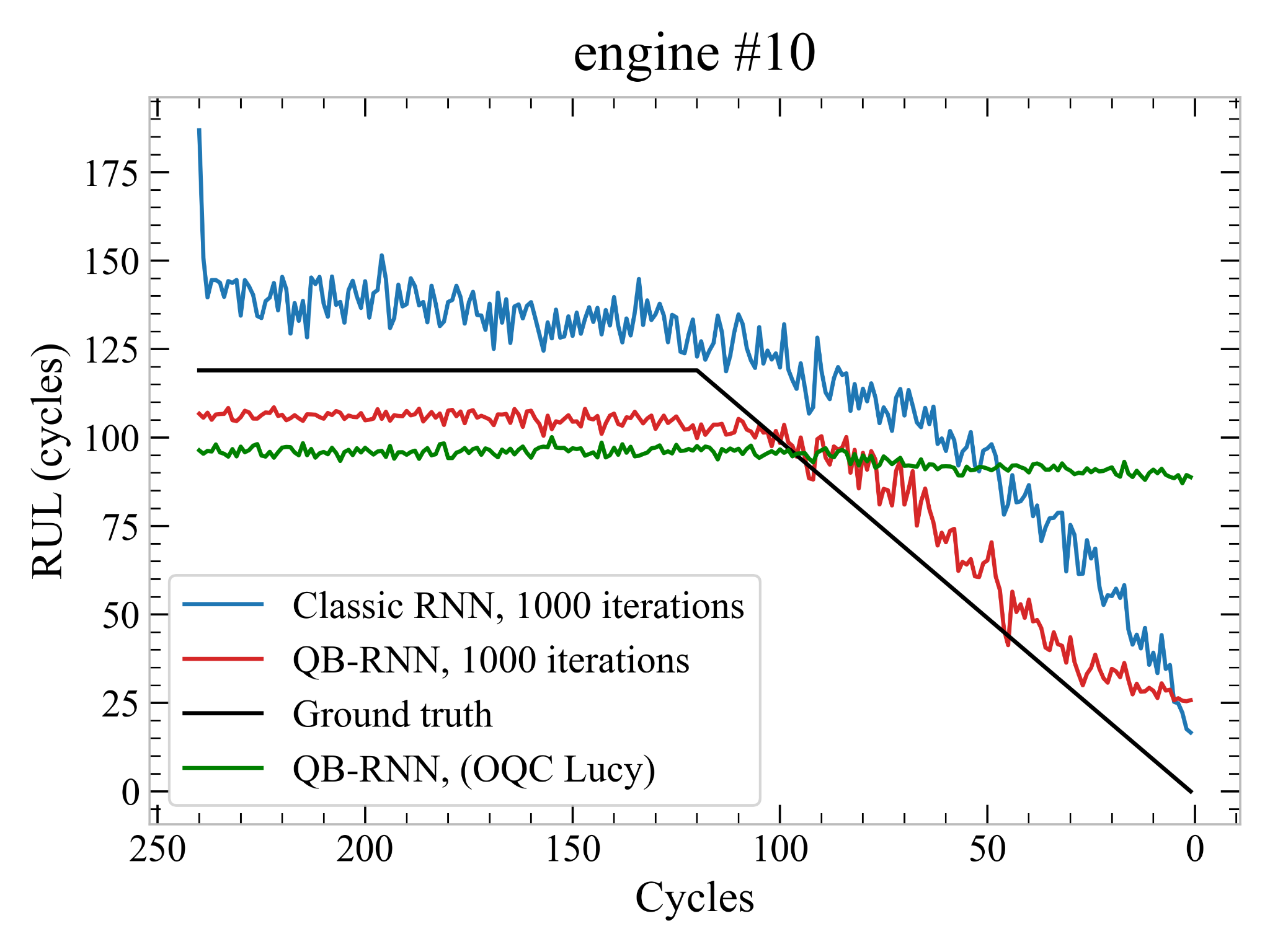
The plot shows the prediction of the models on one of the engine in the training set. The black line is the target line and you can see that QB-RNN generally performs better than RNN, both in terms of distance from the black line and because it is generally underestimating its value rather than overestimating. This is quite of an important point: it is better to underestimate the RUL rather than the opposite!
Funnily enough, when we tried to run QB-RNN on Lucy quantum computer (green line), the results were quite horrendous. This teaches us that we can’t train a Quantum Machine Learning model on an ideal simulator and expect it to work on any device. Ideally we would have liked to train the model on the hardware itself, but the training time turned out to be prohibitive for the limited time we had available.
Conclusion
Our results are interesting, it seems that QB-RNN is performing better than RNN. Does this allow us to claim quantum advantage? Well… Not really. Firstly, by letting the RNN and the QB-RNN run for more training iterations, the results of the former greatly improve. You may be wondering, we didn’t we do so? QB-RNN trains considerably slower than the classic RNN, hence 1000 iterations was the maximum that we could do in the limited time that we had left. By using 1000 iterations for the RNN as well, we wanted to provide a fair comparison, where both algorithms were trained in a similar way. Secondly, the RNN architecture we used is very simple. There is no hidden layer, and it is unfair to compare it with the more sophisticated architecture of the QB-RNN.
Nevertheless, our work is a proof of concept that hybrid quantum neural networks can be successful in training on noisy data and extracting relevant information from them. Quantum machine learning is a relatively new field of research, and I am excited to see how it is going to develop in the next years, when larger and more stable quantum computers will become available.
We were a bit sorry to see our model miserably failing on Lucy, and if we had more time, we would have liked to explore this further, for instance by including the error model of the device into the training of the algorithm. However, the lack of time is probably one of the crucial points of hackathons, and we are happy of what we have accomplished!